 AWS
AWS Microsoft Azure
 Google Cloud

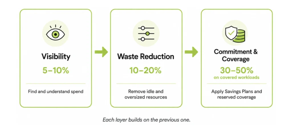
Organizations that complete all three layers can often reduce eligible compute and database costs substantially through waste removal, rightsizing, and commitment discounts; actual total-bill savings vary significantly by workload mix, existing coverage, and implementation scope.
Managing cloud spend remains a top challenge for 85% of organizations, per Flexera’s 2026 State of the Cloud Report and manual optimization efforts can take months to fully implement.
This guide covers:
- The 18 specific practices, organized by layer, that produce measurable savings across AWS, Azure, and GCP.
- An implementation roadmap for choosing which layer to tackle first from tagging audit to continuous optimization.
The short answer
Done together, these can substantially reduce eligible compute and database costs total-bill savings vary by workload mix, existing coverage, and implementation scope.
The sequence matters each layer builds on the previous one, from tagging audit through waste elimination to commitment purchases. And it isn’t a one-time cleanup: coverage needs automated analysis, utilization monitoring, and reassessment as workloads evolve.
The 3 Categories of Cloud
Cost Optimization
In practice, cloud cost optimization falls into three distinct categories. Each builds on the previous one and each unlocks a different level of savings.
| Category | Focus | Illustrative Savings Range* |
|---|---|---|
| Visibility | Cost allocation, tagging, spend tracking | 5–10% |
| Waste Reduction | Idle resources, rightsizing, non-prod scheduling | 10–20% |
| Commitment & Coverage | Savings Plans, RIs, CUDs, coverage rate management | 30–50% (on covered workloads) |
Category 1: Visibility Best Practices
(5–10% Savings)
Practice 1: Identify the Top 3 Services Driving 70–80% of Spend
In nearly every multi-cloud environment, compute (EC2 / Azure VMs / GCE) dominate, databases (RDS, Azure SQL, Cloud SQL) follow, and Kubernetes or storage sits next. As a working rule of thumb, any single service consuming an outsized share of total spend for many teams, 20% or more deserves dedicated optimization modeling.
Before advanced optimization, you should be able to answer:
- What percentage of spend is compute?
- What percentage of compute is on-demand?
- Which region carries the largest baseline load?
Practice 2: Enforce ≥90% Tagging Compliance
Minimum viable tag set: Owner, Environment (prod/staging/dev), Application/workload, Cost center.
If tagging isn’t automated at provisioning time (via Terraform, ARM templates, or policy-as-code using OPA or Sentinel), it will degrade within a quarter. Enforce at deploy time using each cloud’s native guardrails AWS Tag Policies combined with IAM condition keys or AWS Config rules, Azure Policy, or GCP Organization Policies and block non-compliant resources; no soft fails.
Practice 3: Track On-Demand Exposure, Not Just Total Spend
Instead, track what percentage of predictable workloads are still running on on-demand pricing. If 40–50% of baseline compute run on-demand, you are structurally overpaying even if utilization looks healthy.
Illustrative example: $3M annual compute spend × 45% on-demand × 30–50% potential discount = a six-figure optimization opportunity before deleting a single instance. Actual savings depend on workload eligibility, the commitment instruments used, and each provider’s discount rates.
Practice 4: Measure Unit Economics (Cost Per Workload)
Cost per order, cost per API call, cost per inference, cost per GB transferred, these metrics reveal whether spending is scaling efficiently or simply growing. At the FinOps “Run” maturity stage, unit economics become the primary lens for all cloud financial decisions.
Start with one customer-facing service: divide its attributable cloud cost by the relevant output metric (orders, requests, jobs). That ratio is your unit cost baseline. Track it monthly.
Practice 5: Install Anomaly Detection with Action Ownership
Effective anomaly detection requires a threshold definition (e.g., 15% week-over-week increase, an example threshold to tune to your spend profile), an assigned owner, and a defined remediation playbook. Watch for sudden regional expansion, Kubernetes node scaling anomalies, storage growth creep, and commitment coverage dips.
Most anomalies are not catastrophic spikes; they are a slow creep of 3–5% monthly growth that compounds into six figures annually.
Category 2: Waste Reduction
Best Practices (10–20% Savings)
Practice 6: Eliminate Idle and Zombie Resources
Common offenders: instances with 0–5% utilization over 7+ consecutive days, detached EBS volumes, orphaned snapshots, load balancers without active targets, and Kubernetes nodes running without active pods. These are example thresholds that tune them to workload behavior, SLOs, and business criticality. In mid-sized environments, idle resource cleanup alone often reveals mid-five-figure annual savings.
Practice 7: Rightsize Based on Sustained Baseline Utilization
When rightsizing:
- Analyze 30–60 days of historical data
- Review both CPU and memory utilization
- Weight sustained averages over rare peaks but identify what those peaks represent (batch windows, failovers, quarter-end or seasonal traffic) before discounting them
- Evaluate p95 usage separately from steady-state baseline
Average compute utilization varies widely by workload, autoscaling strategy, and infrastructure type, but in many production environments it sits well below provisioned capacity. A practical target for steady-state production workloads is 50–65% utilization, with autoscaling absorbing bursts.
Practice 8: Optimize Kubernetes as a First-Class Cost Driver
- Requests vs. actuals: Use a Vertical Pod Autoscaler (VPA) to tune pod CPU and memory requests against real p95 utilization, note that VPA can evict and restart pods depending on mode, and it interacts with HPA, the Cluster Autoscaler/Karpenter, and pod disruption budgets, so validate before enabling.
- Namespace-level showback: Allocate Kubernetes spend by namespace, team, or workload using labels without it, engineers have no cost feedback loop.
- Bin-packing efficiency: Persistently low node utilization can be a red flag; misconfigured resource requests often inflate cluster sizes but rule out intentional headroom for autoscaling, resilience, or HA requirements before treating it as waste.
- Idle node groups and PVC lifecycle: Enforce TTL-based cleanup on ephemeral PVCs and monitor idle node groups for scale-in opportunities.
Practice 9: Schedule Non-Production Environments Intentionally
Scheduling non-production environments for business hours only (a 40-hour week vs. a 168-hour week) reduces that runtime by more than 75%. Automated shutdown policies for nights and weekends produce immediate savings without performance trade-offs.
Practice 10: Actively Manage Storage, Data Transfer, and Egress Costs
Key actions:
- Set snapshot retention policies (delete snapshots older than 60–90 days unless tagged keep or subject to compliance, legal-hold, backup-dependency, or disaster-recovery requirements)
- Implement lifecycle policies that transition infrequently accessed object storage to lower-cost tiers (e.g., S3 Intelligent-Tiering or Glacier after 30–90 days of inactivity) account for retrieval latency and charges and minimum storage durations (90 days for Glacier Flexible Retrieval, 180 days for Deep Archive) before transitioning
- Review cross-region and cross-AZ data transfer patterns; if inter-region traffic is a material and growing share of total spend, an architecture review is warranted
- Evaluate private links, VPC endpoints, and service-adjacent data placement to reduce NAT and public-routing costs in eligible architectures PrivateLink adds hourly and per-GB processing charges, so model costs before and after rather than assuming savings
Practice 11: Optimize AI/ML and GPU Workloads
AWS Spot Instances including GPU-backed instances are available at discounts of up to 90% compared to on-demand pricing. Spot and preemptible instances require fault-tolerant training pipelines with checkpointing to handle the 2-minute interruption notice AWS issues on a best-effort basis before reclaiming capacity.
Cost-per-inference tracking is the unit economics equivalent for AI workloads: if that number climbs as traffic scales, examine whether value per inference is rising with it unit cost alone doesn’t determine economic viability, but uncontrolled growth erodes margins unless business value grows faster.
Specific actions:
- Use spot/preemptible instances for training jobs with checkpointing enabled
- Right-size inference endpoints using p95 request latency, not peak capacity
- Improve model serving efficiency (batching, caching, quantization) before scaling compute
- Tag all AI/ML resources with a dedicated workload-type: ai-ml tag
Category 3: Commitment & Coverage Practices (30–50% Savings)
When that baseline runs on on-demand pricing, organizations overpay by design. The 30–50% savings in this category apply to covered workloads.
These practices run in order: understand the instruments → model your baseline → purchase in layers → de-risk lock-in → automate → govern and report.
Practice 12: Understand All Commitment Instruments Before You Purchase
| Cloud | Instrument | Discount Range | Flexibility | Best For |
|---|---|---|---|---|
| AWS | Compute Savings Plans | Up to 66% | High (EC2, Fargate, Lambda, all regions) | Dynamic, mixed workloads |
| AWS | EC2 Instance Savings Plans | Up to 72% | Medium (single instance family, single region) | Stable, single-family fleets |
| AWS | Database Savings Plans | Up to 35% | High (eligible engines, instance families, deployment options, all regions) | Managed databases (Aurora, RDS, DynamoDB, ElastiCache, DocumentDB, Neptune, and more) |
| AWS | SageMaker Savings Plans | Up to 64% | Medium (SageMaker usage) | Stable ML workloads on SageMaker |
| AWS | Reserved Instances (Standard) | Up to 72% | Low–Medium | Specific, stable configurations |
| AWS | Spot Instances | Up to 90% | N/A (interruptible) | Fault-tolerant batch and training |
| Azure | Savings Plans for Compute | Up to 65% | High (all VM series, all regions) | Dynamic Azure VM workloads |
| Azure | Savings Plan for Databases | Up to 35% | High (eligible database services, all regions) | Dynamic, multi-service Azure database estates |
| Azure | Reserved VM Instances | Up to 72% (higher with Azure Hybrid Benefit) | Medium (exchanges allowed until Feb 1, 2027; reservations bought before then get one final exchange after that date) | Stable VM configurations |
| GCP | Spend-based CUDs | 28–46% | High (across regions; eligible machine series plus GKE and Cloud Run usage) | Mixed GCP compute |
| GCP | Resource-based CUDs | Up to 55–70% | Low (specific machine family, region) | Stable, single-family Compute Engine |
Sources: Discount ranges per official AWS, Azure, and GCP pricing documentation. Azure exchange policy per Microsoft Cost Management docs (announced July 2026, effective February 1, 2027).
Choose Compute Savings Plans when workloads span multiple regions or you anticipate instance family changes. Choose EC2 Instance Savings Plans when you have a highly stable, single-region, single-family baseline that has been consistent for 6+ months.
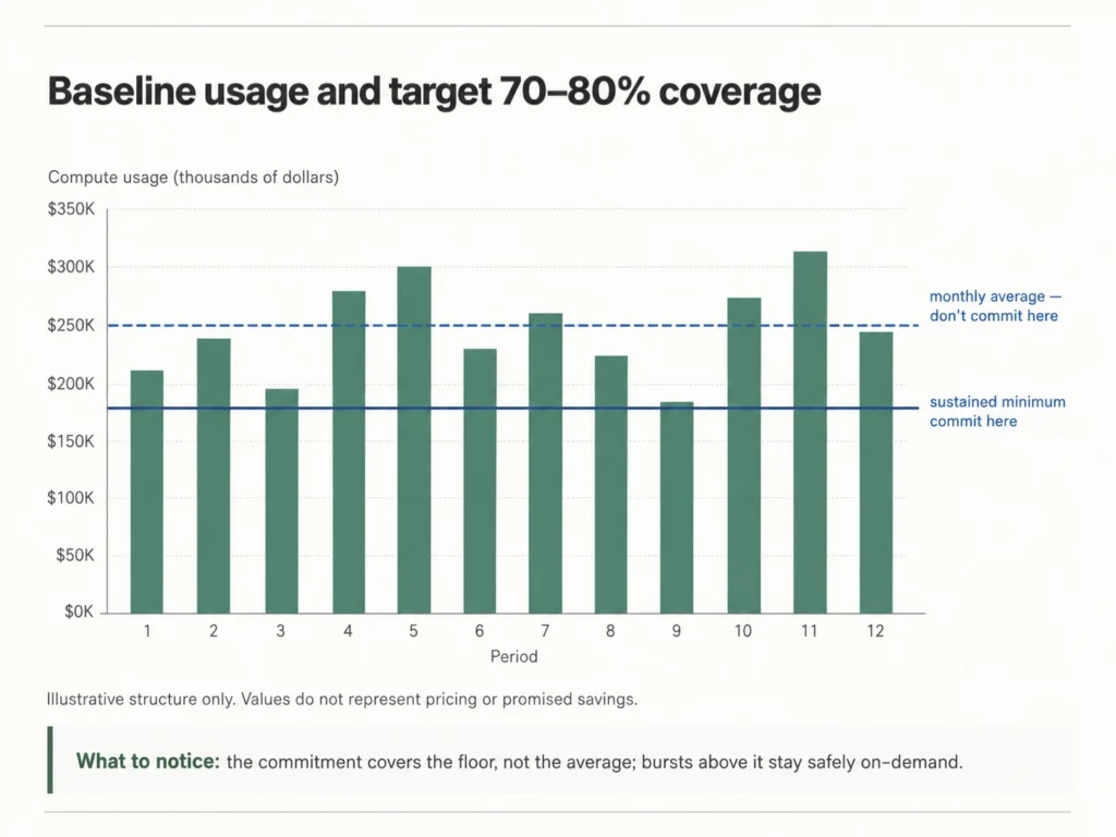
Practice 13: Model Baseline Usage and Target 70–80% Coverage
Model 60–90 days of historical usage at hourly granularity, separating burst traffic from sustained load.
Example: if your monthly compute averages $250K but sustained minimum usage is $180K, target the $180K baseline committing to the full average introduces unnecessary exposure.
As illustrative guardrails rather than industry standards: full 100% coverage is rarely optimal, a 70–80% band is a common working range for stable compute, and many teams start around 70% in the first purchase cycle but the right target for your environment depends on workload predictability, growth trajectory, seasonality, and risk tolerance.
Coverage measures the percentage of eligible usage receiving a commitment discount. AWS, Azure, and GCP each calculate coverage differently, so use each provider’s native coverage definition rather than a single cross-cloud formula.
Directional guardrails (rules of thumb, not hard thresholds):
- Below 60% in a stable environment → likely excessive on-demand exposure
- Above 90% → reassess overcommitment risk
Practice 14: Layer Commitments Across Services Strategically
- Compute workloads (EC2, VMs, GCE)
- Relational databases (RDS, Azure SQL, Cloud SQL)
- Caching services (ElastiCache, Azure Cache)
- Data warehouse platforms (Redshift, BigQuery)
Also read: AWS Savings Plans vs. Reserved Instances: A Practical Guide
Practice 15: Address Lock-In Risk Explicitly
Flex Commitments address this directly. Usage.ai’s Insured Commitments secure the discounts of one- and three-year AWS, Azure, and GCP commitments while reducing risk with terms as short as 30 days.
Cashback protection covers the downside: at the end of each month, any loss where a commitment costs more than the equivalent on-demand usage is calculated, accrued, and paid out to your bank account 90 days after it accrues. With the downside insured, coverage targets can move beyond the conservative levels that lock-in fear typically imposes.
Also read: How to Choose Between 1-Year and 3-Year AWS Commitments
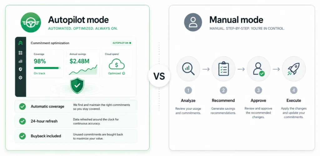
Practice 16: Automate Commitment Analysis and Purchasing
Automated recommendation refresh on a daily cadence allows organizations to adjust to workload changes quickly, prevent sustained on-demand exposure, and maintain target coverage bands consistently.
AWS’s native recommendations are built on billing data that can take up to 24 hours to become available and use fixed multi-day lookback windows, so they can trail your actual usage. A daily refresh cadence closes that gap on a large cloud bill, every day of uncovered baseline compute is a discount you never get back.
Practice 17: Monitor Utilization and Reassess as Architecture Evolves
Key metrics:
- Commitment coverage % (are enough workloads covered?)
- Commitment utilization % (are active commitments being used?)
- On-demand spend ratio (what percentage remains uncovered?)
- Underutilized commitment exposure (are you paying for unused capacity?)
Beyond routine monitoring, certain changes warrant an immediate fresh look at allocation: instance family migrations, region expansion, containerization or Kubernetes adoption, database engine upgrades, and traffic growth or contraction. Coverage that was appropriate six months ago may be misaligned today.
Practice 18: Report Realized Savings in Financial Terms
- Total realized savings vs. prior on-demand baseline
- Service-level breakdown
- Coverage and utilization metrics
- Net savings after fees or program costs
- Month-over-month impact
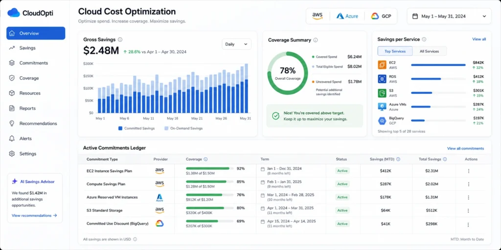
Cloud Cost Optimization
Implementation Roadmap
| Phase | Timeline | Focus | Expected Outcome (illustrative) |
|---|---|---|---|
| Phase 1: Assessment | Week 1–2 | Tagging audit, spend analysis, on-demand exposure calculation | Baseline visibility; identification of top 3 cost drivers |
| Phase 2: Waste Elimination | Month 1 | Idle resource cleanup, rightsizing top 10 instances, non-prod scheduling | 10–20% cost reduction |
| Phase 3: Commitment Strategy | Month 1–2 | Baseline modeling, first commitment purchases at 70% coverage target | 30–50% reduction on covered workloads |
| Phase 4: Continuous Optimization | Ongoing | Daily recommendation cadence, utilization monitoring, coverage drift correction | Sustained savings as workloads evolve |
Conclusion
See how much you’re currently overpaying AWS. Run your free savings calculation in 60 seconds →
Connect in 15 minutes. No contracts, no infrastructure changes. See your savings before committing.
Frequently asked questions
What are the most effective cloud cost optimization best practices?
The most effective cloud cost optimization best practices combine all three layers: (1) establish cost visibility with ≥90% tagging compliance and on-demand exposure tracking; (2) eliminate waste through rightsizing, idle resource cleanup, and non-production scheduling; and (3) align baseline workloads with commitment instruments, with many teams targeting coverage in the 70–80% range for stable workloads. Teams that implement all three layers typically see the largest reductions, with results varying by workload mix, existing coverage, and implementation scope.
How much can you realistically save with cloud cost optimization?
Organizations that optimize only for waste reduction (idle resources, rightsizing) often achieve 10–20% savings. Teams that also optimize commitment coverage ensuring predictable workloads run on discounted instruments can achieve 30–50% reductions on covered workloads. These are illustrative ranges; actual results depend on workload mix, eligibility, and existing coverage.
What is the commitment coverage rate?
Commitment coverage rate is the percentage of eligible baseline cloud spend covered by discounted commitment instruments (Savings Plans, Reserved Instances, CUDs) rather than running at on-demand pricing. AWS, Azure, and GCP each calculate coverage differently, so use each provider's native definition rather than a single cross-cloud formula. A 70–80% band is a common target for stable compute environments, though the right level depends on workload predictability, growth, seasonality, and risk tolerance.
How often should you review cloud costs?
Anomaly detection should run continuously. Commitment coverage and utilization should be reviewed weekly. Comprehensive cost and optimization reviews work best monthly, with commitment strategy reassessments quarterly.
How do spot instances reduce cloud costs?
Spot instances (AWS) and Spot VMs (GCP, the successor to preemptible VMs) offer discounts of up to 90–91% compared to on-demand pricing, in exchange for the possibility of interruption when the cloud provider needs that capacity back. They are well-suited for fault-tolerant batch processing, data pipelines, and AI/ML training with checkpointing enabled. They are generally unsuited to latency-sensitive or stateful production workloads, though mixed-capacity architectures can safely run parts of these systems on Spot.