.png)


Introduction
Public cloud spending is heading toward a massive US $723 billion, but are teams really in control of their costs?
This growth is mostly driven by enterprises moving legacy workloads into AWS, building cloud-native applications, and experimenting with emerging technologies like generative AI. Yet as cloud adoption accelerates, so does the pressure on engineering and FinOps teams to understand whether their AWS environments are truly cost-efficient.
Many organizations measure overall cloud spend, but very few track their AWS Savings Plan KPIs that shed light on efficiency, commitment health, and utilization quality.
Today, where usage patterns shift weekly and architecture changes are frequent, teams need actionable AWS cost-savings metrics to know whether they are capturing expected discounts or leaving money on the table.
This article outlines the seven most important AWS Savings Plan KPIs every FinOps and DevOps team should track to build predictable, measurable cloud efficiency.
%2013%20(17).svg)
Understanding AWS Savings Plan Mechanisms
Before measuring AWS savings plan performance, it’s important to understand what you’re actually measuring. AWS offers multiple ways to reduce compute costs, but each mechanism introduces different levels of flexibility, commitment, and financial risk.
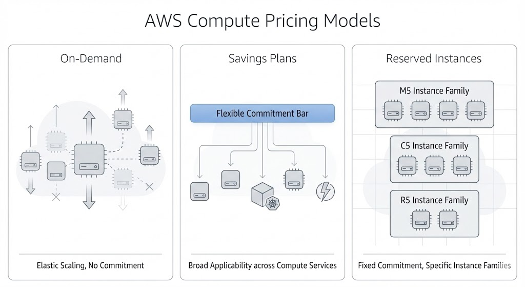
On-Demand (Your Baseline Cost)
On-Demand pricing is the starting point for almost every workload. It offers complete flexibility where you can spin resources up, shut them down, and only pay for what you use. It’s ideal for experimentation and unpredictable patterns, but it’s also the most expensive way to operate long-running workloads. Most savings KPIs compare actual spend to what you would have paid using On-Demand rates.
Savings Plans (Flexible Commitment Discounts)
AWS Savings Plans reduce cost when you commit to a certain amount of compute usage per hour for one or three years. They’re popular because they automatically apply across a wide range of compute services and instance families, which makes them easier to fit to evolving architectures.
For KPI tracking, AWS Savings Plans introduce two central questions:
- How much of your usage is covered?
- Are you consistently using the amount you committed to?
Reserved Instances (More Specific Commitments)
Reserved Instances offer similar discounts but attach those discounts to specific instance families and configurations. They work well for stable, predictable workloads where teams know exactly what they will be running for the long term.
With RIs, it becomes especially important to monitor:
- Whether the environment still matches what you committed to
- How much of the RI inventory is actually being used
- Whether usage patterns have drifted since the commitments were purchased
Also read: AWS Savings Plans vs Reserved Instances: Guide to Buying Commitments
Why a KPI Framework Matters
Commitments don’t guarantee savings by themselves. They create the opportunity for savings and teams only capture those savings when their commitments match their real-world usage. Architectural shifts, seasonal patterns, autoscaling behavior, and right-sizing efforts can all change the shape of your environment month to month.
Without a KPI framework, it’s easy to end up with unused commitments, under-coverage, or inconsistent savings performance. So, these measures are about understanding efficiency, identifying leakage, and ensuring your commitments are working as expected. The seven KPIs in the next section provide a practical, data-driven way to track all of that.
The 7 KPIs That Matter for AWS Savings Plan Success
1. Savings Plans & RI Coverage Percentage
Coverage is the foundational KPI for any AWS savings plan strategy. It measures how much of your compute usage is protected by discounted commitments (i.e., Savings Plans or Reserved Instances) versus how much is still billed at higher On-Demand rates. Even small pockets of uncovered usage can add up quickly, especially in environments that scale dynamically.
Why Coverage Matters
Coverage tells you whether you’re fully leveraging commitment-based discounts. Low coverage typically means:
- You’re paying more than necessary for stable, ongoing workloads.
- Your commitment strategy hasn’t kept up with your actual usage patterns.
Extremely high coverage, on the other hand, can introduce risk if usage suddenly drops.
How to Calculate Coverage
Most teams calculate coverage as the percentage of total compute usage that falls under Savings Plans or RIs during a specific period.
Coverage % = (Committed Usage ÷ Total Compute Usage) × 100
You can express this in terms of spend, hours, or normalized units depending on your internal reporting standards.
Let’s assume in a given month:
- Total compute usage = 10,000 instance-hours
- Hours covered by Savings Plans and RIs = 7,200 instance-hours
Coverage % = (7,200 ÷ 10,000) × 100 = 72%
This means about 72% of your workload benefited from commitment discounts, and the remaining 28% ran on On-Demand pricing.
What Good Looks Like
Healthy coverage varies by environment:
- For stable, predictable workloads, higher coverage is generally safe.
- For highly variable or rapidly changing environments, moderate coverage reduces risk.
- For containerized / autoscaling environments, require more granular, service-level tracking.
The goal should be a consistent match between your commitments and your real usage over time.
Signals to Watch
- Growing pockets of unexpected On-Demand usage
- Coverage dips during migrations or right-sizing efforts
- Seasonal shifts that reduce usage below expected patterns
Coverage is the first and clearest indicator of how well your commitment strategy aligns with real-world behavior. Every other KPI builds on this one.
2. Commitment Utilization Rate
While coverage tells you how much of your environment is protected by commitments, utilization tells you how effectively you’re using what you’ve already purchased. Commitment Utilization Rate measures the percentage of your Savings Plans or Reserved Instances that are actually being consumed by real workloads.
Why Utilization Matters
Commitments create the opportunity for lower costs, but only when workloads consume the capacity you agreed to. Low utilization means you’re effectively paying for unused discounts, and high utilization means your commitments are well aligned with real activity.
This KPI helps teams understand:
- Whether commitments need to be resized
- Whether workloads have moved to new regions / families
- Whether usage has dropped since the commitments were purchased
- Whether commitments are being cannibalized by internal changes (e.g., autoscaling rules, technology shifts)
How to Calculate Utilization (Formula)
Utilization % = (Used Commitment ÷ Purchased Commitment) × 100
This can be measured in:
- Dollar-per-hour commitment amounts (Savings Plans)
- Instance-hours (Reserved Instances)
- Normalized units (for mixed fleets)
Let’s assume, you purchased a Savings Plan committing to $50/hour of compute usage. During this month, your actual compute usage billed under the plan is $42/hour. So,
Utilization % = ($42 ÷ $50) × 100 = 84%
This means you are only using 84% of what you committed to and 16% is the wasted spend for that period.
What Good Looks Like
Utilization targets depend on environment type:
- For stable workloads, 90–100% utilization is usually achievable.
- For variable or seasonal workloads, 70–90% utilization may be safer to reduce risk.
- For rapidly evolving architectures, utilization will swing more, so monitoring weekly or monthly trends becomes important.
High utilization doesn’t always mean “buy more.” It just signals that your commitments are well matched to current patterns.
Signals to Watch
- A sudden dip in utilization after right-sizing or architecture changes
- Commitments tied to legacy instance families or old deployment patterns
- Persistent underutilization on specific services
- Rising On-Demand usage while commitments sit idle
Low utilization is almost always a sign that commitments should be adjusted or that commitments were purchased based on outdated assumptions.
Also read: Save 30-50% on AWS in Under 5 Minutes: The Complete Setup Guide
3. Realized Savings vs Expected Savings
Understanding the difference between expected savings and realized savings is essential for evaluating whether your AWS cost-optimization strategy is actually delivering the results you anticipated. Many teams assume that buying Savings Plans or Reserved Instances guarantees savings, but the financial outcome depends entirely on how consistently those commitments align with your actual usage.
Why This KPI Matters
Expected savings represent the theoretical discount AWS commitments can deliver under perfect usage conditions. Realized savings reflect what you actually saved after real-world fluctuations, like autoscaling, migrations, right-sizing, service changes, and usage dips.
This KPI helps teams answer questions like:
- Are we capturing the savings we planned for?
- How much value are we losing to underutilized commitments?
- Did architecture or usage changes erode our expected benefit?
- Are our forecasts accurate enough to support long-term commitments?
How to Calculate Realized Savings
Realized Savings % = (On-Demand Cost Equivalent – Actual Cost) ÷ On-Demand Cost Equivalent × 100
Where:
- On-Demand Cost Equivalent is what you would have paid without commitments
- Actual Cost is what you actually paid with Savings Plans/RIs applied
Let’s assume for this month, you on-demand cost equivalent is $120,000 and the actual cost (after Savings Plans and RIs) i is $84,000
Realized Savings % = ($120,000 – $84,000) ÷ $120,000 × 100 = 30%
This means, you achieved 30% real savings after commitments were applied. If your procurement model projected 40% savings, you now have a 10-point gap between expectation and reality.
What Good Looks Like
There’s no universal benchmark, but there are certain patterns which you can consider:
- Mature FinOps organizations: Track both expected vs realized savings monthly, and explain deltas.
- Mid-level teams: Focus on realized savings trends to validate purchasing decisions.
- Early-stage teams: Often see large gaps as they calibrate coverage and utilization.
Signals to Watch
- A widening gap between expected and realized savings
- Lower-than-planned savings following a migration or scale-down
- Consistent underutilization of certain commitment families
- A spike in On-Demand spend despite existing commitments
This KPI provides the clearest window into the financial performance of your savings strategy. The next KPI builds on this by measuring how much of the maximum possible discount you’re actually capturing.
4. Savings Efficiency (Discount Capture Rate)
Savings Efficiency measures how effectively your organization captures the maximum possible savings available from commitment-based discounts. Even if coverage and utilization appear healthy, it’s still possible to leave meaningful savings on the table.
This KPI gives teams a clearer view of how much discount value they’re truly capturing compared to what they could have captured with optimally sized commitments.
Why Savings Efficiency Matters
Savings Efficiency cuts through the noise of total spend and provides a clean indicator of discount performance. It helps teams understand:
- How well commitments match usage patterns
- How much of the discount opportunity remains unused
- Whether On-Demand segments are unnecessarily large
- Whether commitments need to be rebalanced or extended
How to Calculate Savings Efficiency
Savings Efficiency % = Realized Savings ÷ Maximum Potential Savings × 100
Where:
- Realized Savings is the actual dollar savings achieved with your current commitments
- Maximum Potential Savings are savings you could have captured if all eligible usage were fully covered and optimally utilized
Let’s assume that your maximum potential savings for this month is $80,000 and the realized savings is $56,000.
Savings Efficiency % = $56,000 ÷ $80,000 × 100 = 70%
This means, your organization captured 70% of the total possible discount value, and 30% of the available savings opportunity remains uncaptured.
What Good Looks Like
There’s no universal benchmark, but there are certain patterns which you can consider:
- 70–90%: Healthy range where most commitments are aligned with usage
- >90%: Strong alignment; often seen in stable, mature FinOps organizations
- <60%: Indicates material inefficiencies that warrant investigation
- Unexpected On-Demand spikes
- Unused commitments
- Mismatched architectures (e.g., shifting to new instance families)
While 100% efficiency is theoretically ideal, the goal should be to minimize inefficiency; not to eliminate it entirely.
Signals to Watch
- An increase in On-Demand spend while commitments remain static
- Rising usage in new services or instance families not covered by commitments
- Decreased usage in areas where commitments were originally sized
- Seasonal patterns that increase the gap between potential and realized savings
Savings Efficiency helps teams identify if their current commitment strategy is optimized or structural adjustments are needed before the next renewal or purchase cycle.
Learn more: How to Choose Between 1-Year and 3-Year AWS Commitments
5. Burndown Forecast Accuracy
Burndown Forecast Accuracy measures how closely your predicted resource usage aligns with actual consumption over time. Since Savings Plans and Reserved Instances are commitments made months or years in advance, forecasting errors can directly impact savings outcomes.
When forecasts are too optimistic, you risk overcommitting; when they’re too conservative, you miss out on deeper discounts. This KPI helps teams evaluate how reliably their forecasting models support long-term commitment decisions.
Why Burndown Forecast Accuracy Matters
EC2 fleets, container workloads, and service adoption patterns rarely stay static. Architecture changes, right-sizing efforts, seasonal patterns, and even organizational restructuring can all affect how much compute your environment consumes.
Accurate forecasting allows teams to:
- Size commitments with confidence
- Avoid unnecessary exposure to usage dips
- Anticipate when commitments should be extended, reduced, or rebalanced
- Communicate expected savings performance to finance and leadership
How to Calculate Burndown Forecast Accuracy (Formula)
There are several ways to measure forecast accuracy, but a simple and effective method is Percentage Error. It measures how close actual usage was to your predicted value.
Forecast Accuracy % = (1 – |Actual Usage – Forecasted Usage| ÷ Forecasted Usage) × 100
Let’s assume your forecast predicted 50,000 instance-hours for the month, and your actual usage came in at 46,000 instance-hours.
- Error = |50,000 – 46,000| = 4,000
- Error rate = 4,000 ÷ 50,000 = 0.08 (8%) Forecast accuracy = (1 – 0.08) × 100 = 92%
This means your forecast was 92% accurate, which is strong. Forecasts with >85–90% accuracy generally support healthy commitment decisions.
What Good Looks Like
Forecast accuracy varies widely depending on workload type:
- Stable, predictable workloads: Often achieve 90%+ accuracy
- Containerized or autoscaling systems: Typically fall into the 75–90% range
- Environments undergoing migrations or modernization: Accuracy drops temporarily until usage stabilizes
What matters is not a single accuracy score, but the trend. Improving accuracy over time signals maturity in both engineering and FinOps processes.
Signals to Watch
- Forecasts consistently overestimating usage (risk of overcommitment)
- Forecasts consistently underestimating usage (missed savings opportunities)
- Sudden accuracy drops following architectural changes
- Divergence between team-level forecasts and organization-wide trends
A reliable forecast is the backbone of long-term AWS savings strategy. The next KPI focuses on workload-level cost performance which is another critical dimension of savings measurement.
6. Cost per Functional Unit (Workload-Level Efficiency)
While most AWS savings plan KPIs focus on commitments and compute efficiency, Cost per Functional Unit zooms in on the cost of delivering value to the business. This KPI measures how much it costs to serve a single unit of work, such as a request, job, user session, pipeline run, or message processed regardless of the underlying architecture.
This shifts the conversation from infrastructure costs to workload performance, making it easier for engineering and product teams to understand whether efficiency is improving or declining over time.
Why Cost per Functional Unit Matters
It is possible for overall cloud spend to go down while workload efficiency actually gets worse, or vice versa. This KPI controls for noise by tying cost directly to output.
Teams use it to answer questions like:
- Are we spending more or less to deliver the same amount of work?
- Did recent architecture changes improve efficiency?
- Are traffic spikes driving costs proportionally, or disproportionately?
- Which services deliver the best cost-to-value ratio?
How to Calculate Cost per Functional Unit
The formula varies by workload, but the structure remains the same:
Cost per Functional Unit = Total Cost of Workload ÷ Total Units of Output
Where “units of output” may be:
- API requests
- Active users
- Build minutes
- Messages processed
- Jobs completed
- Data ingested
The KPI adapts to any workload where output can be measured.
Let’s assume that a service processes 200 million API requests per month and its total monthly cost (compute + storage + data transfer) is $40,000.
Cost per Request = $40,000 ÷ 200,000,000 = $0.0002 per request
This means that if last month the service cost $0.00025 per request, then efficiency has improved. If the value rose, something regressed, so, maybe your performance tuning, scaling rules, or infrastructure configuration might need review.
What Good Looks Like
“Good” is highly workload-specific, but the trends matter more than the raw numbers. Efficient workloads usually show:
- Stable or declining cost per unit as they scale
- Predictable variation when traffic increases or decreases
- Noticeable improvements after optimization efforts
- Early signals when regressions occur (e.g., memory bloat, suboptimal autoscaling, retried requests)
Cost per functional unit becomes extremely powerful when trended over time because it highlights both operational improvements and architectural inefficiencies.
Signals to Watch
- Cost rising faster than workload output
- Large discrepancies between similar services (e.g., two APIs doing similar work)
- Efficiency regressions following deployments or configuration changes
- Unexpected increases in supporting services (e.g., data transfer, storage IO)
This KPI helps engineering and FinOps teams speak the same language, the cost of delivering value. The final KPI adds an often overlooked dimension—data transfer and retrieval.
7. AWS Data Transfer & Retrieval Cost KPIs (The Hidden Savings Gap)
While most AWS savings plan discussions focus on compute, data transfer and retrieval costs are often the silent contributors to rising cloud bills. In many organizations, these costs grow faster than compute itself, especially when architectures become more distributed, services communicate more frequently, or data pipelines expand.
This KPI helps teams measure how efficiently data moves across services, regions, and storage layers, and how these patterns impact their overall savings strategy.
Why Data Transfer & Retrieval KPIs Matter
Even if your compute commitments are perfectly optimized, unexpected data movement can cost the savings you expected to capture. The following are some common patterns to look for:
- High inter-AZ traffic in multi-AZ deployments
- Cross-region replication and failover
- Microservices that communicate excessively
- S3 retrieval fees from frequent access patterns
- Egress costs from analytics or external integrations
These costs don’t show up in commitment KPIs, but they directly influence the true efficiency of your workloads.
How to Calculate Data Transfer Cost per Unit
There are several ways to track this, but a simple, workload-inclined KPI is:
Data Transfer Cost per Unit = Total Data Transfer Cost ÷ Total Volume of Data Moved
You can apply this formula per workload, per environment, or per service.
Let’s assume a data processing pipeline transfers 150 TB per month, and the associated transfer and retrieval charges total $7,500.
Cost per TB = $7,500 ÷ 150 = $50 per TB
This means, if the cost per TB jumps from $50 to $70 next month, the increase may come from routing inefficiencies, unnecessary cross-AZ movement, aggressive replication settings, or new retrieval patterns.
What Good Looks Like
Because data patterns vary widely, there isn’t a single benchmark. However, efficient environments typically show:
- Stable or predictable cost per TB for the same workload
- Wide gaps in cost that can be traced to architectural decisions (e.g., replication, routing)
- Lower transfer costs when data locality is optimized
- Lower retrieval costs when storage tiers align with access frequency
The goal shouldn’t just be to reduce data transfer, but also to understand when and why it happens, and how it impacts overall savings performance.
Signals to Watch
- Spikes in inter-AZ transfer after scaling events
- High retrieval costs due to frequently accessed S3 objects stored in infrequent access tiers
- Unexplained cross-region replication charges
- Egress cost growth outpacing traffic growth
- Pipelines or microservices with unusually high data-shuffling patterns
Data transfer and retrieval costs often represent the missing piece in savings analysis. Compute commitments may be optimized, but shifting data patterns can quietly chip away at realized savings and distort workload efficiency metrics.
Common Mistakes Organizations Make When Tracking AWS Savings Plan KPIs
Below are some of the most common pitfalls FinOps and engineering teams encounter when tracking AWS savings plan, and why these mistakes can quietly cost otherwise solid optimization efforts.
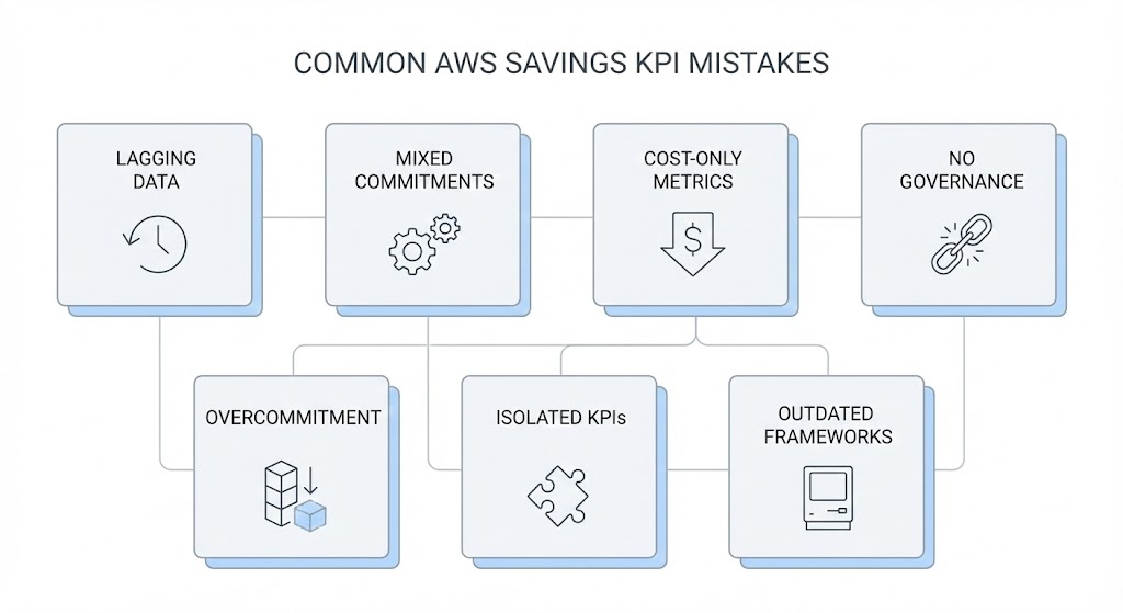
1. Relying on Lagging Billing Data
Many teams base KPIs on delayed billing data, which means commitment decisions are tied to outdated usage patterns. In fast-changing environments, this leads to misaligned commitments, late detection of utilization drops, and savings projections that don’t match reality.
2. Treating All Commitments Equally
Savings Plans and Reserved Instances behave differently, yet some organizations group them together as a single metric. This masks important differences in flexibility, risk, and applicability, making coverage and utilization KPIs less accurate and harder to act on.
3. Measuring “Cost” but Ignoring “Efficiency”
A workload costing less this month doesn’t automatically mean it became more efficient. Without metrics like cost per request or cost per job, organizations miss operational regressions and misinterpret savings that are really the result of traffic changes and not optimization.
4. Lacking Cross-Functional Governance
KPIs fail when engineering, finance, and platform teams interpret them differently or make decisions in isolation. Without shared assumptions and coordinated ownership, commitment strategies drift, forecasts diverge, and savings outcomes become unpredictable.
5. Overcommitting Without a Risk Buffer
Chasing high coverage or high utilization can push teams into overcommitment, especially in variable or evolving environments. Without a buffer for seasonal or architectural changes, organizations face underutilized commitments and financial exposure when usage dips.
6. Tracking KPIs in Isolation
Coverage, utilization, efficiency, and forecasting aren’t separate stories. Evaluating each KPI on its own hides the relationships between them, making it harder to see issues like misaligned commitments or architectural inefficiencies.
7. Not Updating KPIs as Architecture Evolves
Cloud environments change constantly, but KPI frameworks often remain static. When teams don’t revisit what they measure or how they measure it, they end up tracking outdated metrics that no longer reflect how workloads behave or where costs originate.
How Usage.ai Enhances AWS Savings Plan KPIs
After establishing a strong KPI framework, the next step is ensuring those KPIs translate into consistent, predictable savings. This is where Usage.ai provides a measurable advantage.
By automating commitment decisions, refreshing recommendations daily, and offering cashback-assured coverage, Usage.ai strengthens the exact KPIs FinOps teams rely on to assess the health of their savings strategy.
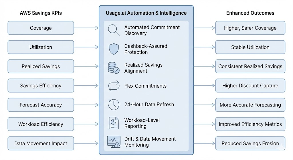
1. Improving Coverage Through Automated Discovery
Usage.ai continuously scans billing and usage to identify where Savings Plans or RIs can safely increase coverage. Instead of relying on lagging or static recommendations, Usage.ai updates insights every 24 hours, helping teams maintain coverage levels that match actual usage patterns.
2. Protecting Utilization with Cashback Assurance
One of Usage.ai’s most unique strengths is its cashback-assured commitment model. If commitments become underutilized due to shifting workloads, Usage.ai pays customers real cash back,effectively reducing the financial risk of utilization drops. This allows teams to achieve higher utilization safely, without fear of overcommitting.
3. Strengthening Realized Savings Quality
Because Usage.ai charges only a percentage of realized savings, its incentives are aligned with actual KPI performance. Teams gain clarity into the true financial impact of their commitments, and Usage.ai helps ensure that realized savings remain close to expected savings over time.
4. Increasing Savings Efficiency with Flex Commitments
Flex Commitments provide Savings Plan–like discounts without long-term lock-in. This gives teams discount coverage even as architectures shift, instance families change, or workloads scale unpredictably.
5. Boosting Forecast Accuracy with Fresh, High-Frequency Data
AWS-native recommendations can lag several days. Usage.ai’s 24-hour refresh cycle helps teams base forecasts and commitment decisions on the most current usage patterns available. This reduces the risk of overcommitting during usage peaks or undercommitting during dips.
6. Supporting Workload-Level Efficiency Metrics
With detailed reporting and transparency features, Usage.ai helps organizations break down savings and commitments by service, team, or workload. This enables more accurate cost-per-unit calculations and highlights where efficiency is improving or regressing.
7. Minimizing Savings Erosion from Data Movement & Drift
By monitoring commitment coverage and usage alignment daily, Usage.ai helps reduce leakage that often emerges from architectural drift, such as shifts to new instance families, right-sizing, or increasing data transfer patterns that distort the savings picture.
Conclusion
What separates mature cloud cost practices from reactive ones is consistency. When these KPIs are reviewed regularly and trended over time, they provide a reliable foundation for smarter commitments.
As cloud environments continue to evolve, the organizations that treat savings as a measurable, data-driven discipline will be the ones that maintain both financial efficiency and architectural agility.
%2022%20(7).svg)
Frequently Asked Questions
1. What are the most important AWS Savings Plan KPIs to track?
The essential AWS Savings Plan KPIs include: coverage percentage, commitment utilization rate, realized vs expected savings, savings efficiency, burndown forecast accuracy, cost per functional unit, and data transfer/retrieval cost KPIs.
2. How often should FinOps teams review AWS Savings Plan KPIs?
Most teams review Savings KPIs monthly, with weekly or daily checks for fast-changing environments. More dynamic workloads benefit from higher-frequency reviews to detect utilization drops or cost anomalies early.
3. What causes low utilization of Savings Plans or Reserved Instances?
Low utilization typically comes from architecture changes, workload right-sizing, usage drops, shifting to new instance families, or services migrating across regions or platforms. Any change that reduces the footprint of the resources your commitments were sized for can cause underutilization.
4. What is a good coverage percentage for AWS Savings Plans?
There’s no universal target, but many stable workloads maintain 70–90% coverage successfully. Highly variable or seasonal environments often choose more moderate coverage to avoid risk.
5. How do I know if I’m overcommitted on AWS?
You may be overcommitted if utilization consistently stays below expectations, realized savings trend downward, or workloads shrink without corresponding adjustment of commitments. Forecasting errors and unexpected architectural changes are common triggers.
6. Why do AWS forecasting errors impact savings?
Forecasting errors affect commitment sizing. If forecasts overestimate usage, you risk underutilized commitments. If they underestimate, you miss available discounts. High forecast accuracy leads to more predictable savings and fewer surprises in coverage or utilization.
7. Why do data transfer and retrieval costs matter for AWS savings?
Data transfer and S3 retrieval fees can consume a significant portion of cloud spend and often grow faster than compute usage. If these costs rise unexpectedly, they can reduce overall workload efficiency and distort savings metrics.
8. How does cost per functional unit improve AWS savings visibility?
Cost per functional unit ties cloud spend to output (e.g., cost per request or cost per job), making it easier to see whether efficiency is improving. It exposes patterns that raw spend cannot, like regressions after deployments or architecture decisions that increase cost per unit.